How Does AI Work? A Plain-English Guide to How Machines Learn

Artificial intelligence powers modern spam filters, navigation routing, and conversational assistants. Yet most explanations remain vague metaphors or jump straight into calculus. This guide details the exact computational mechanics: how algorithms extract patterns from data, how neural networks adjust internal weights, and how large language models generate text token by token.

Included below is an arithmetic walkthrough of a single neuron’s calculations, a breakdown of the six-stage AI pipeline, transformer self-attention mechanics, and physical deployment constraints.

Key Takeaways

• Pattern Learning: AI discovers statistical regularities across data to classify, predict, or generate content without hard-coded rules.
• Training vs. Inference: Training tunes billions of parameters to minimize loss; inference runs the frozen model on new inputs in production.
• Autoregressive Text: LLMs generate one token at a time based on prior context, explaining both fluency and hallucinations.
• Optimization: Backpropagation uses calculus gradients to systematically update weights via gradient descent.
• Operational Realities: Production systems require rigorous drift monitoring and substantial compute infrastructure.

How Does AI Work? The Short Answer

At its computational core, artificial intelligence combines three ingredients: massive training datasets, statistical learning algorithms, and high-performance compute hardware executing billions of matrix multiplications per second.

During training, an algorithm processes input examples, produces predictions, compares them against ground-truth labels via a loss function, and updates internal parameters—weights and biases—to reduce error. Over millions of iterations, the model converges on representations that generalize to unseen data.

Much like a child learning to identify dogs through repeated visual exposure and feedback rather than an exhaustive anatomical manual, machine learning infers probabilistic patterns directly from examples.

The broad field of what artificial intelligence is encompasses machines emulating cognitive functions, with machine learning and deep learning serving as its core data-driven subfields.

From Rules to Learning: How AI Moved Beyond Hand-Written Code

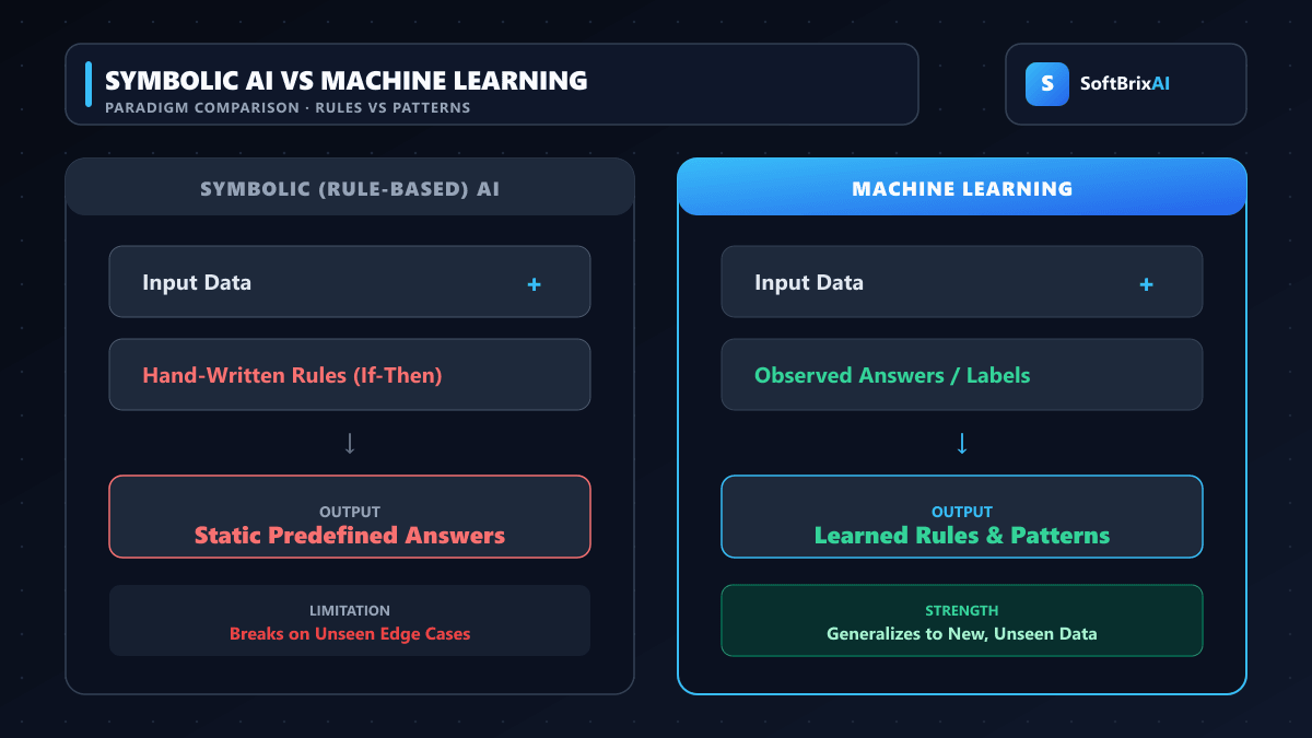Figure 1: Symbolic rule-based systems execute deterministic if-then logic, whereas machine learning algorithms infer probabilistic decision rules directly from data.

Early AI relied on explicit conditional rules authored by human engineers—known as symbolic AI or GOFAI. A legacy spam filter used deterministic heuristics (flagging “FREE MONEY” from unknown senders), while medical expert systems chained together nested if-then rules.

While effective in predictable environments, symbolic systems failed when confronted with real-world variance. Spammers bypassed filters using misspellings (“FR3E M0NEY”), requiring constant manual rule updates.

Machine learning inverted this paradigm. Instead of hand-coding logic, engineers feed labeled datasets to machine learning algorithms, which infer statistical decision boundaries autonomously. Analyzing millions of emails, models discover complex, non-linear signals—combining header anomalies, character n-grams, and dispatch timestamps—far beyond human intuition.

Dimension	Rule-Based (Symbolic) AI	Machine Learning
Logic Origin	Programmers author explicit if-then rules	Algorithms infer mathematical patterns from data
Handling Novel Inputs	Rigid; fails unless covered by existing rules	Flexible; interpolates within learned feature distributions
Explainability	High; decision trees and rules are human-readable	Variable; deep neural networks operate as black-box representations
Primary Cost Driver	Engineering hours to author and maintain rules	Data acquisition, labeling infrastructure, and GPU compute
Everyday Example	Tax software logic, deterministic financial audits	Modern spam filters, Netflix recommendation engines

Deterministic logic still runs plenty of critical software today. Tax software, compliance audits, and safety interlocks rely on fixed logic because absolute predictability matters more than flexibility. Modern enterprise products frequently combine both approaches: deterministic code enforces hard compliance guardrails, while machine learning handles probabilistic judgment calls.

The AI Pipeline: How an AI System Is Built, Step by Step

Every AI system, whether predicting loan defaults or generating software code, moves through the same six-stage engineering lifecycle.

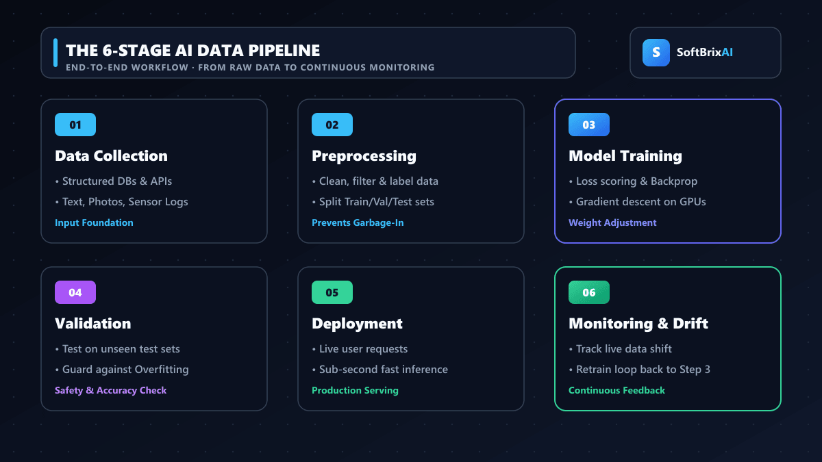Figure 2: The end-to-end AI engineering lifecycle, spanning data preparation, model optimization, validation gates, high-concurrency deployment, and continuous drift monitoring.

1. Data Collection

Models learn entirely from training samples. Teams gather structured relational tables or unstructured media (documents, audio, video)—which comprises over 80% of enterprise information—spanning historical transaction logs or web-scale text tokens.

2. Data Preprocessing

Engineers clean raw data by imputing missing values, deduplicating records, filtering noise, and normalizing numerical scales. Teams scaling architectures leverage custom AI software development to automate data workflows. Data is partitioned into training (70–80%), validation (10–15%), and test (10–15%) subsets.

3. Model Training

In this optimization phase, data batches pass through the architecture, a loss function quantifies error against ground truth, and optimizers (Adam, SGD) update parameters via backpropagation. Models train over multiple epochs across GPU/TPU clusters.

4. Validation and Evaluation

Engineers evaluate against validation sets to prevent overfitting—memorizing training noise rather than learning general patterns. The final model is benchmarked on unseen test data for accuracy, subgroup fairness, and inference latency.

5. Model Deployment and Inference

Validated models are deployed via REST APIs, microservices, or edge runtimes. Production inference evaluates fresh inputs through frozen weights in milliseconds, executing millions of daily requests at optimized operational costs.

6. Monitoring and Retraining

Because real-world distributions shift over time (data and concept drift), engineering teams continuously monitor prediction confidence and accuracy metrics. Automated pipelines trigger periodic retraining, standardized via enterprise MLOps services.

How Does Machine Learning Work?

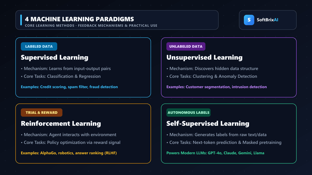Figure 3: The four primary learning paradigms in machine learning categorized by their feedback loops, data dependencies, and commercial applications.

Machine learning algorithms optimize mathematical functions to map input features to output targets without explicit hard-coding. The four primary learning paradigms differ in their feedback mechanisms and data requirements.

Supervised Learning Explained

Supervised learning pairs inputs with verified labels ($x \rightarrow y$) to train mapping functions. It handles two primary problem types:

• Classification: Assigning inputs to discrete categories (e.g., spam detection, disease diagnosis).
• Regression: Predicting continuous values (e.g., financial revenue forecasting, asset valuation). Supervised models power most enterprise applications, from credit scoring to payment risk assessment.

Unsupervised Learning

Unsupervised learning analyzes unlabeled datasets ($x$) to discover latent patterns and geometric structures:

• Clustering (e.g., K-Means): Segmenting user cohorts based on interaction patterns.
• Dimensionality Reduction (e.g., PCA): Compressing wide feature spaces while retaining core mathematical variance.
• Anomaly Detection (e.g., Isolation Forests): Detecting cyber intrusions diverging from baseline traffic.

Reinforcement Learning

Reinforcement learning optimizes an autonomous agent’s policy through trial and error within an environment. The agent executes actions, evaluates numerical rewards or penalties, and converges on long-term reward-maximizing strategies. DeepMind demonstrated this with AlphaGo in 2016; commercial deployments include robotics path planning and datacenter energy optimization.

Self-Supervised Learning: The Method Behind Modern LLMs

Self-supervised learning extracts training targets directly from raw data by masking parts of the input sequence. In language modeling, algorithms predict masked or subsequent tokens across trillions of text samples. Bypassing manual annotation bottlenecks, self-supervision enables web-scale pretraining for foundation models like GPT, Claude, and Gemini.

Learning Paradigm	Training Data	Feedback Mechanism	Typical Tasks	Production Example
Supervised	Labeled ($x, y$)	Explicit ground-truth error	Classification, regression	Fraud scoring, credit underwriting
Unsupervised	Unlabeled ($x$)	Inherent data density and clustering	Clustering, anomaly detection	Customer segmentation, cyber intrusion detection
Reinforcement	Environment states	Dynamic reward and penalty signals	Policy optimization, sequential actions	Autonomous robotics, AlphaGo
Self-Supervised	Unlabeled with masking	Internal token reconstruction loss	Representation pretraining	Next-token prediction in modern LLMs

What Is a Neural Network?

An artificial neural network (ANN) is a machine learning model built from interconnected layers of simple computational units, called artificial neurons, that pass numerical values to one another. Each connection carries an adjustable weight that modulates signal strength, and learning consists of systematically tuning those weights.

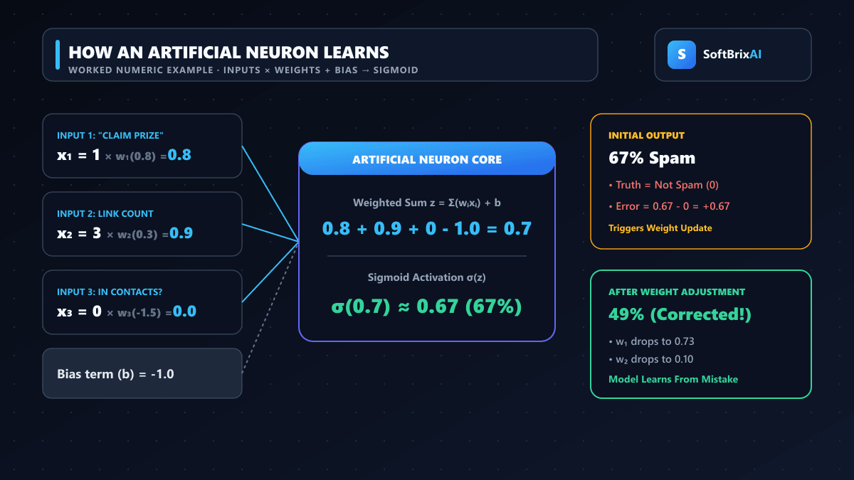Figure 4: Detailed arithmetic trace of a single artificial neuron calculating weighted inputs, applying a sigmoid activation, computing prediction error, and updating internal weights via gradient descent.

Neurons, Weights, and Layers

Neural networks structure artificial neurons across three functional tiers:

1. Input Layer: Ingests normalized numerical features or embeddings.
2. Hidden Layers: Intermediate representations applying non-linear transformations across dozens or hundreds of stacked layers.
3. Output Layer: Generates target predictions (class probabilities or continuous scalars).

Each neuron multiplies inputs ($x_i$) by weights ($w_i$), adds a bias ($b$), and applies an activation function ($f$): $z = \sum_{i=1}^{n} w_i x_i + b, \quad \hat{y} = f(z)$

Activation functions (ReLU, Sigmoid, GELU) introduce non-linearity. Without non-linear activations, multi-layer networks collapse mathematically into single linear regressions, unable to solve non-linear problems.

A Worked Example: One Neuron Learning to Spot Spam

To understand how weights adjust during training, consider a concrete arithmetic trace of a single artificial neuron evaluating whether an email is spam based on three input features:

• $x_1 = 1.0$: Contains the promotional phrase “claim prize” (1 = yes, 0 = no)
• $x_2 = 3.0$: Total count of embedded external links (3 links)
• $x_3 = 0.0$: Sender appears in recipient contacts (1 = yes, 0 = no)

Step 1: Forward Pass Calculation

Assume the neuron begins with initial weights and a bias: $w_1 = 0.8$, $w_2 = 0.3$, $w_3 = -1.5$, and $b = -1.0$.

The neuron computes the linear combination $z$: $$z = (1.0 \times 0.8) + (3.0 \times 0.3) + (0.0 \times -1.5) + (-1.0) = 0.8 + 0.9 + 0.0 - 1.0 = 0.7$$

The sum $z = 0.7$ passes through the standard logistic sigmoid function $\sigma(z) = \frac{1}{1 + e^{-z}}$: $$\hat{y} = \sigma(0.7) = \frac{1}{1 + e^{-0.7}} \approx \frac{1}{1 + 0.4966} \approx 0.668 \quad (66.8%)$$

The neuron generates an initial 66.8% probability that the email is spam.

Step 2: Loss Computation

Suppose the true label indicates this email was a legitimate newsletter requested by the user ($y = 0.0$). The prediction was incorrect. Using squared error loss ($L = \frac{1}{2}(\hat{y} - y)^2$), the prediction error is: $$\text{Error} = \hat{y} - y = 0.668 - 0.0 = 0.668$$

Step 3: Gradient Calculation and Weight Update

To adjust each parameter, the training algorithm applies the calculus chain rule to calculate the partial derivative of loss with respect to each weight ($\frac{\partial L}{\partial w_i} = (\hat{y} - y) \times \hat{y}(1 - \hat{y}) \times x_i$).

Evaluating the sigmoid derivative: $$\sigma’(z) = \hat{y}(1 - \hat{y}) = 0.668 \times (1 - 0.668) \approx 0.2218$$

Calculating the gradient factor $\delta$: $$\delta = (\hat{y} - y) \times \sigma’(z) = 0.668 \times 0.2218 \approx 0.1482$$

With a learning rate $\eta = 0.1$, the parameters update via gradient descent ($w_{\text{new}} = w_{\text{old}} - \eta \frac{\partial L}{\partial w}$):

• Weight $w_1$ Update: $\frac{\partial L}{\partial w_1} = 0.1482 \times 1.0 = 0.1482 \implies w_1^{\text{new}} = 0.8 - (0.1 \times 0.1482) \approx 0.785$
• Weight $w_2$ Update: $\frac{\partial L}{\partial w_2} = 0.1482 \times 3.0 = 0.4446 \implies w_2^{\text{new}} = 0.3 - (0.1 \times 0.4446) \approx 0.256$
• Weight $w_3$ Update: $\frac{\partial L}{\partial w_3} = 0.1482 \times 0.0 = 0.0 \implies w_3^{\text{new}} = -1.5 - 0.0 = -1.500$
• Bias $b$ Update: $\frac{\partial L}{\partial b} = 0.1482 \times 1.0 = 0.1482 \implies b^{\text{new}} = -1.0 - (0.1 \times 0.1482) \approx -1.015$

Step 4: Verification of Updated Parameters

Re-running the same email through the updated neuron: $$z_{\text{new}} = (1.0 \times 0.785) + (3.0 \times 0.256) + (0.0 \times -1.500) - 1.015 = 0.538$$ $$\hat{y}_{\text{new}} = \sigma(0.538) = \frac{1}{1 + e^{-0.538}} \approx 0.631 \quad (63.1%)$$

In a single training step, the neuron reduced its spam probability from 66.8% to 63.1%. When repeated across millions of emails and scaled across billions of connected neurons, these micro-adjustments converge into highly accurate classification systems.

Backpropagation Explained

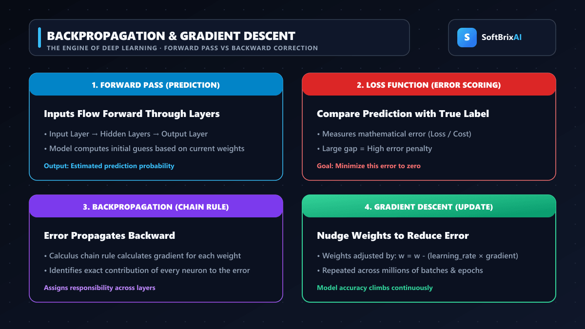Figure 5: The closed-loop optimization cycle in deep neural networks: forward activations compute loss, while backpropagation calculates exact gradients to guide parameter convergence.

Determining how early hidden weights contribute to output error requires backpropagation. Popularized by Rumelhart, Hinton, and Williams in 1986 (Nature), backpropagation applies the calculus chain rule backwards from the loss output through all hidden layers to calculate partial derivatives ($\frac{\partial L}{\partial w_{ij}}$).

These gradients dictate parameter adjustment directions. Optimizers like AdamW apply updates concurrently across all layers with each data batch until the model converges.

What Is Deep Learning?

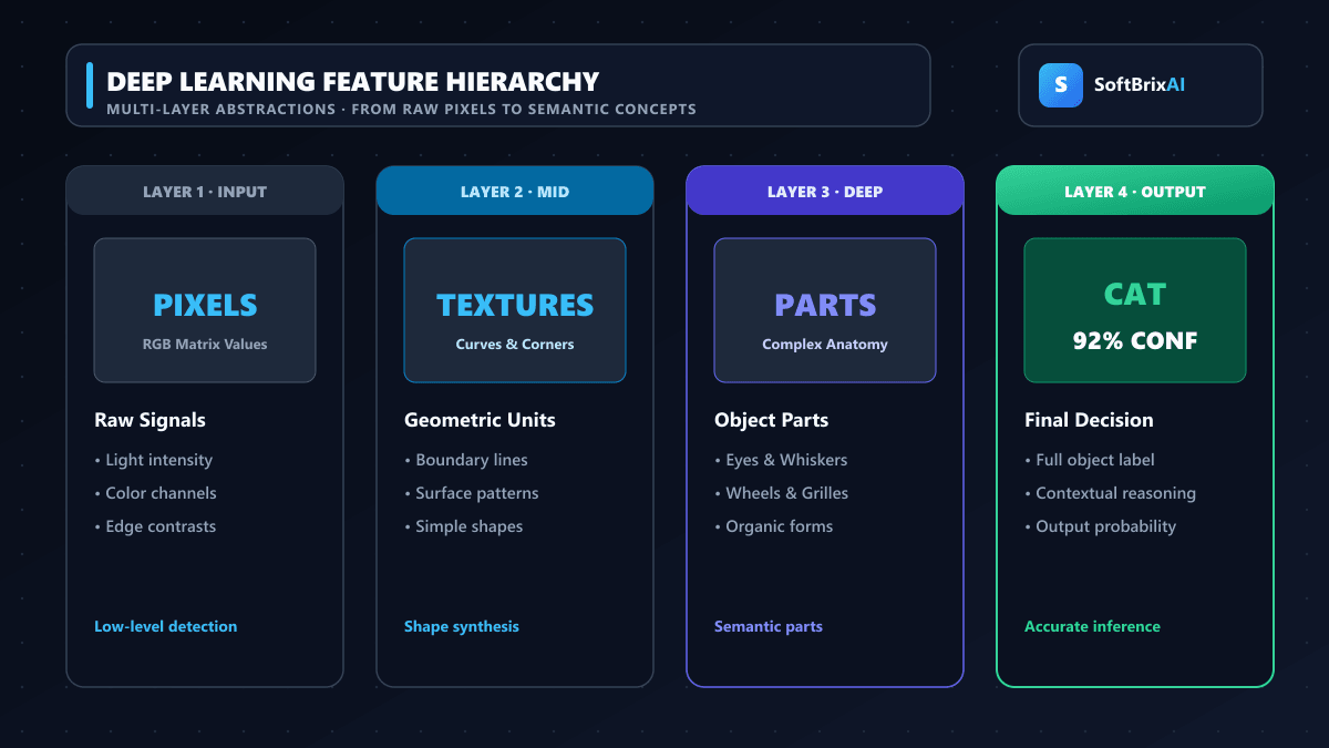Figure 6: Hierarchical representation learning in deep convolutional networks, progressing from raw sensory pixels to semantically meaningful object classification.

Deep learning utilizes neural networks with many hidden layers to extract hierarchical abstractions directly from raw sensory data, eliminating manual feature engineering:

• Early Layers: Detect low-level primitives (edges, pixel gradients).
• Intermediate Layers: Combine primitives into textures and contours.
• Deeper Layers: Assemble contours into semantic object components (wheels, eyes).
• Output Layer: Outputs target classifications (pedestrian, sedan).

The deep learning revolution accelerated in 2012 when AlexNet won ImageNet via GPU training, decisively surpassing hand-crafted algorithms. Modern transformers scale this layered representation across hundreds of billions of parameters.

How Do Large Language Models Work?

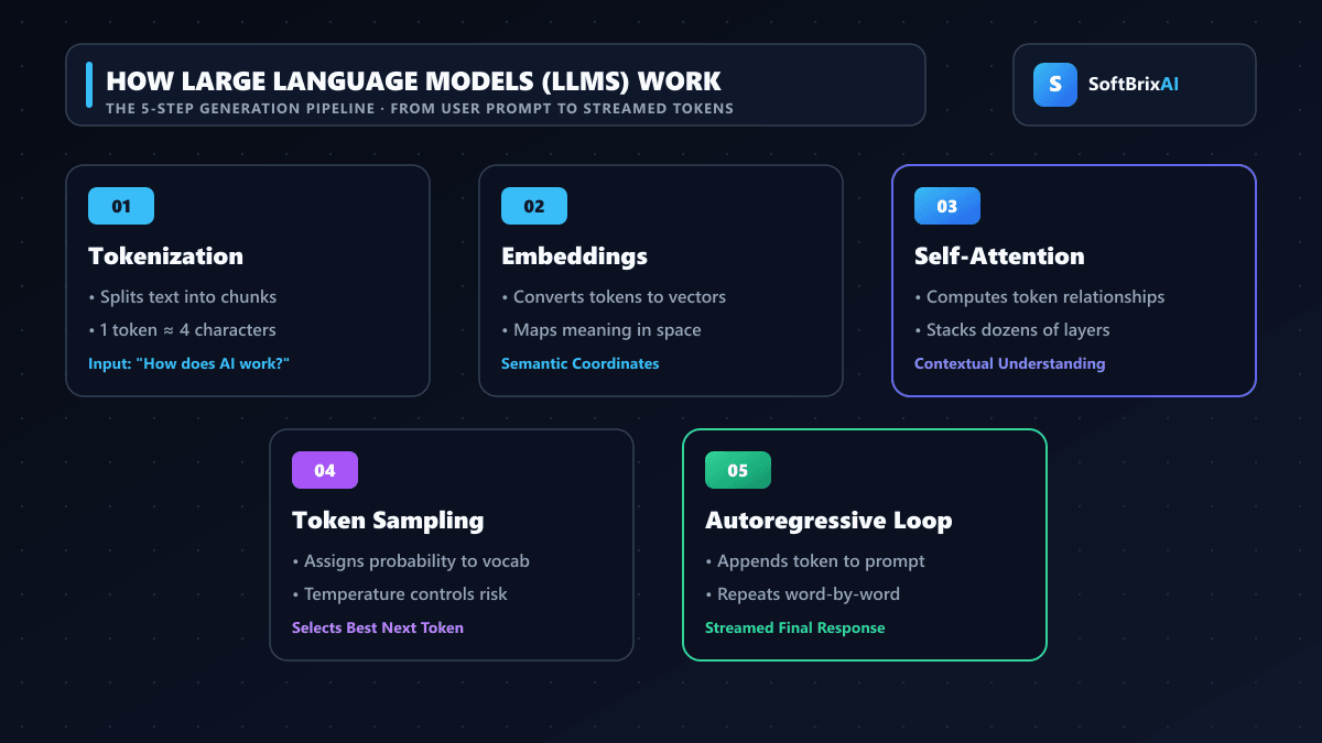Figure 7: The five architectural phases of large language model text synthesis, from lexical tokenization to probabilistic token sampling and autoregressive decoding.

Frontier models like GPT-5.5, Gemini, and Claude synthesize text autoregressively, predicting one token at a time based on preceding context across five stages:

Step 1: Tokenization

Text is segmented into sub-word tokens via Byte-Pair Encoding (BPE). In English, a token averages four characters (~0.75 words). Each token maps to an integer index within the model’s vocabulary (typically 32,000–128,000 entries).

Step 2: Vector Embeddings

Token integers map to continuous vectors in high-dimensional semantic space (e.g., 4,096 dimensions). Words with related meanings cluster together geometrically, while positional encodings inject sequence order.

Step 3: Transformer Attention Mechanism

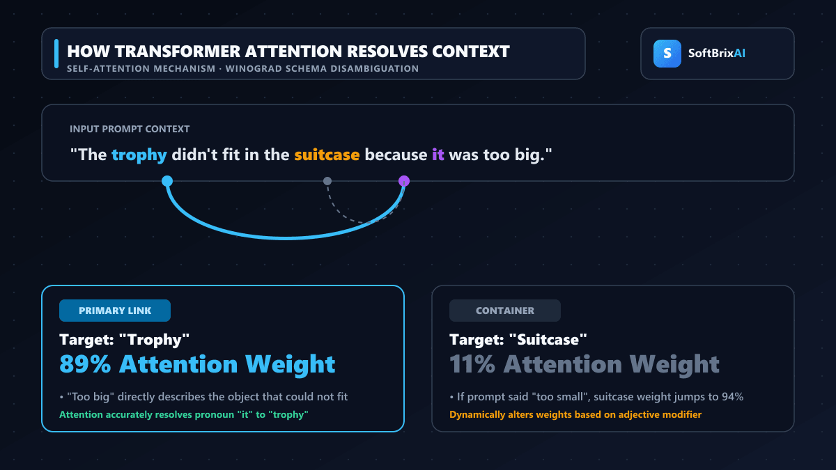Figure 8: Self-attention weights dynamically connecting relational context across token sequences to resolve ambiguous grammatical references.

Introduced by Vaswani et al. in 2017 (“Attention Is All You Need”), multi-head self-attention computes relationships across all tokens simultaneously using Query ($Q$), Key ($K$), and Value ($V$) projections: $\text{Attention}(Q, K, V) = \text{softmax}\left(\frac{QK^T}{\sqrt{d_k}}\right)V$ In “The trophy didn’t fit in the suitcase because it was too large,” attention assigns high weights between “it” and “trophy,” resolving syntactic ambiguity mathematically.

Step 4: Next-Token Sampling

The output layer converts logits to probabilities via softmax. Decoding hyperparameters control sampling:

• Temperature: Lower values ($T \approx 0.2$) produce deterministic, focused text; higher values ($T \approx 0.8$) yield creative variety.
• Top-p (Nucleus): Restricts selection to the smallest token pool with cumulative probability exceeding $p$ (e.g., 0.9). Selected tokens are appended to context, looping until an end-of-sequence marker (<EOS>) triggers.

Step 5: Pretraining, SFT, and RLHF

1. Self-Supervised Pretraining: Ingests trillions of tokens to learn linguistic syntax and world knowledge.
2. Supervised Fine-Tuning (SFT): Demonstrates conversational problem-solving via expert dialogues.
3. RLHF / Direct Alignment: Optimizes models against human preference rewards to ensure safety and helpfulness.

Why LLMs Hallucinate

LLMs optimize for linguistic plausibility rather than ground truth. When parameter representations lack clear factual data, they generate confident, grammatically convincing fabrications. Systems counter this with retrieval-augmented generation (RAG), grounding prompts with verified external datastores.

How Does Generative AI Work Beyond Text?

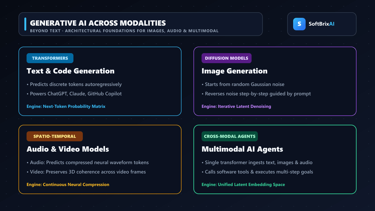Figure 9: Foundational generative AI architectures across modalities, highlighting the technical transition from unimodal models to tool-calling multimodal agents.

Beyond text, generative AI spans diverse data modalities:

• Diffusion Models: Models like Stable Diffusion and Sora learn to reverse Gaussian noise degradation. At inference, they denoise random latent static guided by text embeddings to render images and video.
• Audio Synthesis: Transformers predict discrete acoustic tokens to synthesize speech and music with natural inflection.
• Multimodal Models: Unified architectures (GPT-4o, Gemini 2.5) ingest text, audio, and visual patches within shared transformer backbones.
• Agentic AI: Coupling foundation models with API calling, scratchpads, and execution loops enables autonomous agents to complete multi-step software tasks.

Other Core Disciplines Inside AI

Beyond generative language and vision systems, artificial intelligence comprises several foundational technical branches:

• Natural Language Processing (NLP): Encompasses computational linguistics tasks including named entity recognition, sentiment analysis, and machine translation.
• Computer Vision (CV): Algorithms that extract structural meaning from visual inputs, powering autonomous driving and medical imaging. Explore deeper technical mechanics in our guide on how AI visual search works.
• Pattern Recognition in Speech: Converts acoustic waveforms into frequency spectrograms, using deep convolutional and recurrent networks to map acoustic patterns directly to phonemes and text.
• Autonomous Robotics: Combines computer vision, kinematic path planning, and reinforcement learning to enable physical robots to manipulate objects and navigate dynamic environments.

Types of Artificial Intelligence

Artificial intelligence systems are classified primarily through two complementary frameworks: capability (the breadth of cognitive tasks a system can perform) and functionality (how an architecture manages memory and models external agents).

For an exhaustive analysis of narrow AI (ANI), artificial general intelligence (AGI), superintelligence (ASI), and the four functional types, see our dedicated guide on types of artificial intelligence.

A Short History of How AI Came to Work This Way

The computational architecture of modern artificial intelligence evolved through five decisive milestones:

Year	Milestone	Architectural Significance
1950	Turing’s Imitation Game	Alan Turing published “Computing Machinery and Intelligence”, proposing the Turing Test and framing machine intelligence through empirical behavior.
1986	Backpropagation Formalization	Rumelhart, Hinton, and Williams demonstrated that backpropagation and gradient descent could train multi-layered neural networks.
2012	AlexNet ImageNet Victory	AlexNet utilized GPU acceleration to win the ImageNet challenge, proving deep convolutional networks decisively outperformed classical computer vision.
2017	The Transformer Architecture	Vaswani et al. introduced self-attention in “Attention Is All You Need”, establishing the core architectural foundation for all modern LLMs.
2022	ChatGPT & Reinforcement Learning	OpenAI paired instruction-tuned transformers with RLHF, bringing generative AI into mainstream consumer software.

AI vs Human Decision Making

Evaluating artificial intelligence alongside human cognition reveals distinct operational trade-offs:

Factor	Artificial Intelligence Systems	Human Decision Makers
Processing Speed	Evaluates millions of records per second	Bounded by biological attention
Consistency	Applies identical weights to identical inputs	Influenced by fatigue and context
Generalization	Degrades on out-of-distribution inputs	Navigates novel tasks via intuition
Ethical Reasoning	Lacks moral and contextual awareness	Synthesizes empathy and moral nuance
Explainability	Functions as mathematical black boxes	Articulates subjective rationale
Bias	Amplifies training corpora bias	Subject to social correction

This complementary balance underpins augmented intelligence: leveraging algorithms for high-throughput pattern recognition while maintaining human governance over critical decisions.

How AI Works in the Real World

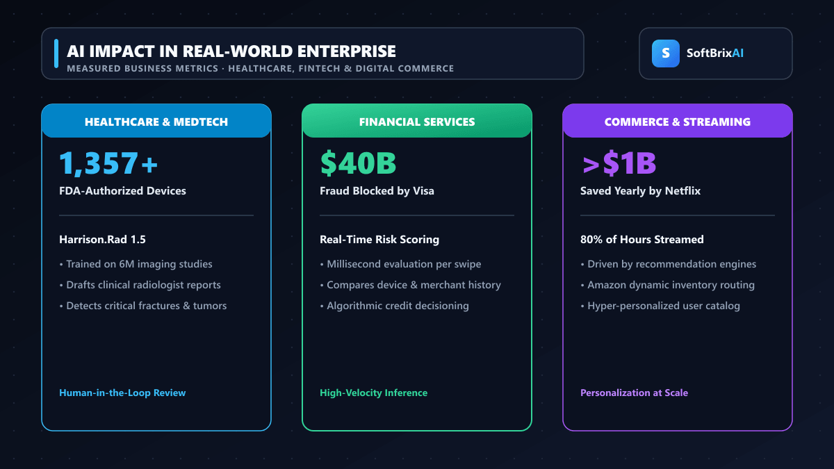Figure 10: Production impact of artificial intelligence across regulated healthcare diagnostics, high-throughput fraud prevention, and personalized commerce engines.

Production artificial intelligence systems execute mission-critical workflows across diverse global sectors:

• Clinical Healthcare: Computer vision models assist radiologists by triaging medical imaging studies. By early 2026, the FDA had authorized over 1,350 AI-enabled medical devices, accelerating diagnostic workflows while requiring clinical confirmation.
• Financial Security: Payment networks evaluate transactions within milliseconds using supervised classifiers that score incoming requests against rolling behavioral baselines. Visa reported its fraud mitigation models prevented over $40 billion in fraudulent transactions in 2024.
• Digital Commerce & Media: Collaborative filtering and deep retrieval models personalize streaming and shopping feeds. Netflix engineers reported their recommendation architecture saves over $1 billion annually by preserving subscriber engagement.

For an extensive analysis of industry use cases across enterprise manufacturing, logistics, and software engineering, see our comprehensive guide on what artificial intelligence is.

AI Challenges and Limitations

Deploying production artificial intelligence introduces significant technical and operational constraints:

Model Hallucinations and Reliability

Sequence models optimize for statistical plausibility rather than truth. Stanford HAI’s 2026 benchmarks documented hallucination rates spanning 22% to 94% across leading foundation models, necessitating retrieval grounding and human verification.

Bias Amplification and Concept Drift

Models systematically reproduce historical disparities present in training data. Additionally, post-launch data and concept drift erode prediction accuracy as real-world behaviors diverge from training baselines.

Compute Infrastructure and Energy Consumption

Scaling frontier models demands immense power. The International Energy Agency (IEA) documented datacenter electricity consumption at 415 TWh in 2024, projecting growth to 945 TWh by 2030 driven by AI clusters.

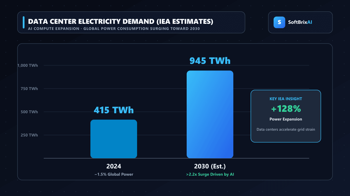Figure 11: Global data center electricity demand projections through 2030 based on International Energy Agency (IEA) findings, driven by AI accelerator clusters.

Black-Box Opacity

High-parameter networks lack clear mechanistic interpretability. While feature attribution (SHAP) and attention maps provide partial insight, tracing causal prediction chains remains challenging in regulated sectors.

Responsible AI and AI Governance

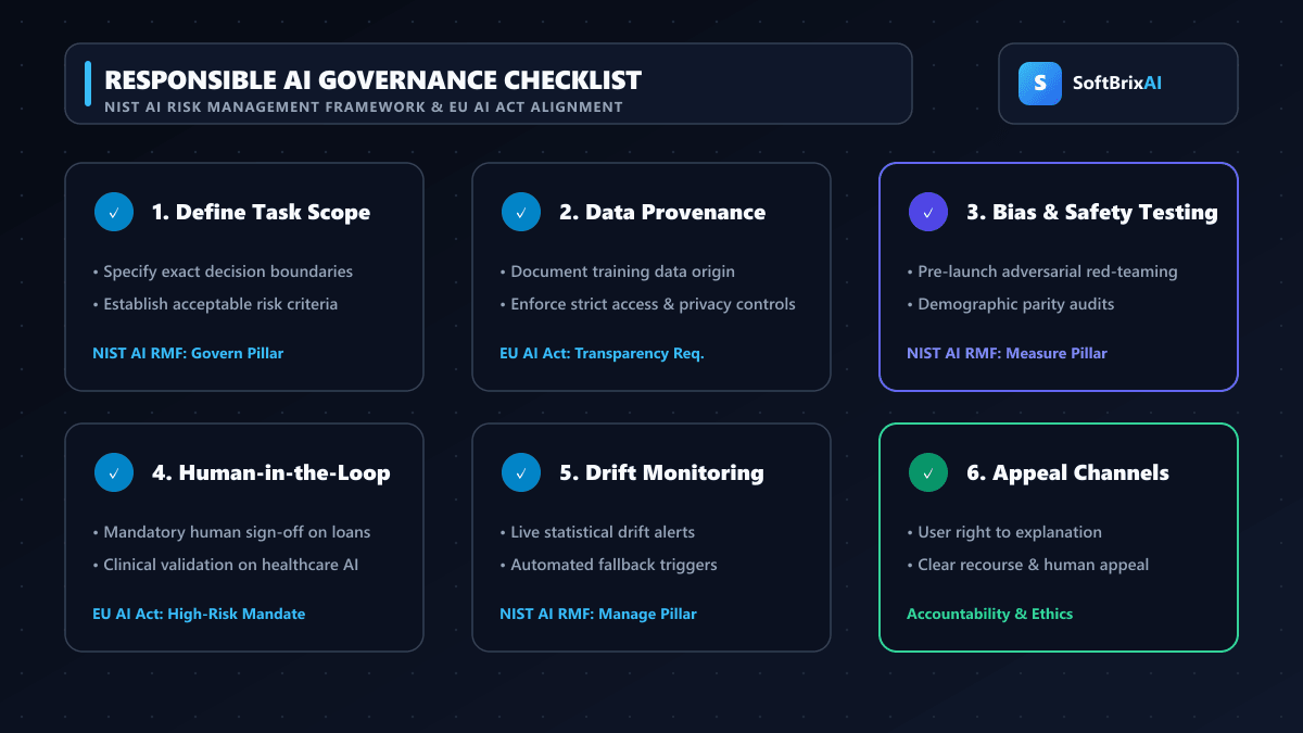Figure 12: Enterprise AI governance operational checklist aligned with the NIST AI Risk Management Framework and EU AI Act risk-tier obligations.

Deploying machine learning responsibly requires systematic operational guardrails. International governance frameworks—including the NIST AI Risk Management Framework and the binding requirements of the European Union’s EU AI Act—mandate thorough data provenance audits, pre-deployment bias testing, continuous drift monitoring, and guaranteed human-in-the-loop escalation channels for high-risk applications. For an enterprise-level analysis of compliance roadmaps, consult our pillar guide on what artificial intelligence is.

Conclusion

Understanding how artificial intelligence works dispels the mystique surrounding modern machine learning. At every scale—from a single artificial neuron adjusting weights to separate spam to multi-billion-parameter transformers generating software code—AI operates on an optimization loop: ingesting data, measuring prediction error against objective loss functions, and iteratively updating mathematical parameters via backpropagation.

As enterprise adoption accelerates, the engineering focus shifts from pure model size to data quality, inference efficiency, and systemic governance. To deepen your understanding of the broader technological landscape, explore our guides on what artificial intelligence is, the distinct types of artificial intelligence, and our detailed comparison of AI vs machine learning vs deep learning.

Frequently Asked Questions

How does AI learn from data?

AI models learn through mathematical optimization. Algorithms process inputs, generate predictions, compare them against target labels using a loss function, and update internal weights via backpropagation and gradient descent to minimize error over successive iterations.

What is the difference between AI training and AI inference?

Training is the compute-intensive phase where models learn internal weights from massive datasets. Inference is the operational phase where the frozen model processes unseen inputs in real time.

How do neural networks use backpropagation?

Backpropagation applies the calculus chain rule backwards from the output loss through hidden layers, calculating partial derivatives for each weight to guide gradient descent updates.

How does an LLM like ChatGPT generate responses?

LLMs synthesize text autoregressively token by token. Multi-head self-attention models contextual relationships across tokens, projecting probabilities over the vocabulary to sample the next token.

Why do large language models hallucinate?

LLMs optimize for linguistic plausibility rather than factual verification. Gaps in training data lead to fluent but inaccurate text, which enterprises mitigate via retrieval-augmented generation (RAG).

What is the role of an activation function in a neural network?

Activation functions (ReLU, Sigmoid, GELU) introduce non-linearity. Without them, stacking multi-layer networks collapses mathematically into a single linear regression, preventing models from learning complex patterns.

References

1. Turing, A. M. (1950). “Computing Machinery and Intelligence.” Mind, 59(236), 433–460.
2. Rumelhart, D. E., Hinton, G. E., & Williams, R. J. (1986). “Learning representations by back-propagating errors.” Nature, 323, 533–536.
3. Krizhevsky, A., Sutskever, I., & Hinton, G. E. (2012). “ImageNet Classification with Deep Convolutional Neural Networks.” NeurIPS.
4. Vaswani, A., et al. (2017). “Attention Is All You Need.” Advances in Neural Information Processing Systems.
5. Brown, T., et al. (2020). “Language Models are Few-Shot Learners.” arXiv:2005.14165.
6. Ouyang, L., et al. (2022). “Training language models to follow instructions with human feedback.” NeurIPS.
7. Stanford Institute for Human-Centered Artificial Intelligence. (2026). The 2026 AI Index Report.
8. McKinsey & Company. (2026). The State of AI.
9. International Energy Agency. (2026). Energy and AI: Executive Summary.
10. National Institute of Standards and Technology. (2023). AI Risk Management Framework (NIST AI RMF 1.0).
11. European Parliament. (2024). The European Union Artificial Intelligence Act.
12. Silver, D., et al. (2016). “Mastering the game of Go with deep neural networks and tree search.” Nature, 529, 484–489.