How Does AI Visual Search Work? A 2026 Engineering Guide ...

By Umar Abbas, Principal AI Architect, SoftBrixAI

A shopper photographs a chair in a hotel lobby and gets back twelve buyable products that look like it. No words were typed. Nothing was tagged. The system had never seen that chair, that lighting, or that camera angle before.

Most explanations of AI visual search stop at “the AI compares your image to a database.” That sentence is not wrong, but it hides every decision that determines whether the feature ships or stalls. This guide walks the full path from a raw photo to a ranked result set, and it spends most of its length on the parts that break: retrieval at scale, filtering, re-ranking, and the gap between a shopper’s phone camera and clean product photography.

Key Takeaways

Visual search replaces lexical matching with vector proximity. The query image becomes a list of numbers, and retrieval means finding the closest other lists of numbers.

Production systems are never one step. They run object detection, visual query encoding, approximate nearest neighbor retrieval, filtering, and re-ranking as separate stages with separate failure modes.

Exact nearest neighbor search does not scale. Approximate methods such as HNSW trade a small amount of recall for logarithmic query complexity, and binary quantization cuts storage further.

Filtering has to happen inside retrieval, not after it. Post-filtering a top-k result set is the most common reason a visual search returns an empty page.

The hardest engineering problem in ecommerce visual search is not the model. It is keeping embeddings synchronized with a catalog whose SKUs, variants, and inventory status change hourly.

How AI visual search differs from keyword search

Keyword search matches strings. A shopper types “brass floor lamp,” the engine looks up documents containing those tokens or their close relatives, and ranking proceeds from there. The entire system rests on somebody having written the words down. Product photography that nobody described in text is invisible to it.

AI visual search removes that dependency. The query is the image itself, and matching happens in a geometric space rather than a lexical one. Both the query image and every catalog image are converted into fixed-length numeric vectors, and similarity becomes a distance measurement. Two products that look alike land near each other in that space whether or not anyone ever tagged them with the same words. This is what people mean by semantic image matching, and it is why visual search can surface a product whose listing says “accent seating” when the shopper photographed something they would have called an armchair.

The scale of the behavior shift is documented. Google reported roughly 3 billion Google Lens searches per month in May 2021 (Google, 2021). By October 2024 the company put the figure at nearly 20 billion visual searches per month, with 20 percent of Lens searches described as shopping related (Google, 2024). The same trajectory shows up in Google’s conversational surface: AI Mode reached 1 billion monthly users roughly a year after launch, with queries more than doubling every quarter since (Google, 2026).

For teams building on this, the practical consequence is that visual searchers arrive with different intent than search users typing keywords. They usually already know what the object looks like and are trying to find where to buy it, or something close to it. That intent shapes every downstream ranking decision, and it is why the retrieval and ranking stages described below cannot be borrowed wholesale from a text search stack. If you are weighing that architectural decision, our AI software development practice treats visual search as a retrieval problem first and a model problem second.

The visual search pipeline, stage by stage

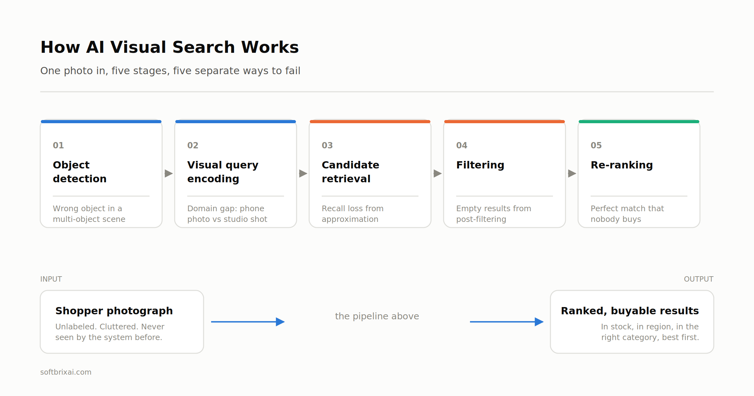
A working visual search system is a pipeline, not a call to a model. Collapsing it into one step is the single most common error in how this technology gets described, and it leads directly to underestimating the build.

Stage	What happens	Primary failure mode
Object detection	Locate and crop the item of interest inside a cluttered photo	Wrong object chosen in a multi-object scene
Visual query encoding	Convert the crop into a fixed-length embedding	Domain gap between user photos and catalog imagery
Candidate retrieval	Find the nearest vectors in the indexed catalog	Recall loss from aggressive approximation
Filtering	Remove items that are out of stock, out of region, or out of category	Empty result sets from post-filtering
Re-ranking	Reorder candidates using business rules and behavioral data	Visually perfect results that nobody buys

Each stage has its own latency budget, its own evaluation metric, and its own way of failing quietly. A system can have an excellent embedding model and still return useless results because the filter runs in the wrong place. A system can have flawless retrieval and still lose revenue because it ranks a discontinued SKU first.

The stages are also independently swappable, which matters for how the work gets sequenced. Object detection can start as a simple center crop and improve later. The embedding model can be replaced without touching the retrieval layer, provided the vector dimensionality stays constant or the index is rebuilt. Re-ranking can begin as a hard-coded business rule and grow into a learned model once there is click data to train on. Teams that treat the whole thing as one monolithic AI feature tend to over-scope the first release and ship nothing.

Google’s own architecture illustrates how far the pipeline concept extends. Rather than running a single lookup, Google describes a visual search fan-out that runs multiple queries in the background to build a deeper understanding of what is in an image, layering Lens and Image Search with Gemini 2.5’s multimodal capabilities to recognize secondary objects alongside primary subjects (Google, 2025). Dounia Berrada, a Senior Engineering Director on Search, characterized the approach plainly: the system “is basically doing a dozen searches for you in the time it takes to do one” (Google, 2026).

How images become vectors

Everything downstream depends on this stage producing a representation where visual similarity equals numeric proximity. Get it wrong and no amount of retrieval engineering compensates.

Vision transformers and patch sequences

For most of the 2010s, neural feature extraction on images meant convolutional neural networks. That changed with the Vision Transformer, which showed that a pure transformer applied directly to sequences of image patches could match state-of-the-art convolutional networks on classification benchmarks while requiring substantially fewer computational resources to train (Dosovitskiy et al., Google Research, 2020). The paper’s title captures the mechanism: an image is worth 16x16 words. The picture is cut into fixed-size patches, each patch is linearly projected into a token, and the transformer’s attention mechanism does the rest.

This matters for visual search because attention-driven visual search behaves differently from convolutional pipelines. A multi-scale feature pyramid in a CNN builds representations hierarchically from local texture upward. Attention lets the model relate distant regions of an image directly, which helps when the distinguishing feature of a product is its overall silhouette rather than a local pattern.

Contrastive image and text training

The Vision Transformer produces good deep learning descriptors, but it still needs a training objective that makes the resulting vectors useful for search rather than classification. Contrastive Language-Image Pre-training supplied one. CLIP was trained on 400 million image and text pairs collected from the internet, learning to predict which caption belongs with which image. The result transferred to more than 30 computer vision datasets without task-specific training, and matched the ImageNet accuracy of the original ResNet-50 without using any of the 1.28 million labeled examples that model was trained on (Radford et al., OpenAI, 2021).

Two properties make CLIP-style image embeddings the default starting point for visual search. First, zero-shot image classification means the model handles product categories it was never explicitly trained on, which is essential for a catalog that adds new categories continuously. Second, because images and captions share one space, the same index supports cross-modal search fusion: a shopper can start from a photo and refine with text, or vice versa. That image caption grounding is what powers “find this, but in green” interactions.

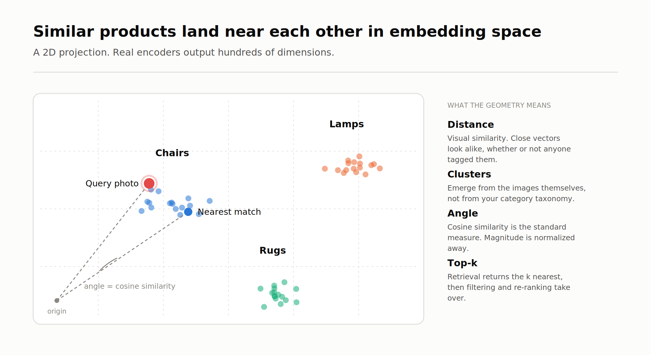
A 2D projection of an embedding space. Clusters form from the images themselves, not from the catalog taxonomy.

What changed after CLIP

The contrastive recipe has since been refined. SigLIP replaced CLIP’s softmax normalization with a sigmoid loss operating on individual image and text pairs, removing the need for a global view of pairwise similarities during training. The practical payoff was efficiency: the authors reported 84.5 percent ImageNet zero-shot accuracy trained on four TPUv4 chips in two days, and found that batch sizes beyond roughly 32,000 delivered diminishing returns (Zhai et al., Google Research, 2023).

For a team choosing an encoder in 2026, the decision is rarely about squeezing out the last point of benchmark accuracy. It is about embedding dimensionality, inference cost per image, and license terms, because those three determine what the storage and retrieval layer will cost for the next several years.

Finding matches at scale: approximate nearest neighbor search

Once every product image is a vector, search becomes a similarity search problem: given a query vector, find the closest vectors in the catalog. Cosine similarity is the usual distance measure. The naive implementation compares the query against every indexed vector, which is exact and completely impractical past a few tens of thousands of items.

Approximate nearest neighbor methods trade a controlled amount of recall for a large speedup. Hierarchical Navigable Small World graphs are the dominant approach. HNSW incrementally builds a multi-layer structure of proximity graphs, assigning elements to layers with an exponentially decaying probability distribution and beginning each search at the sparse upper layers before descending. The authors reported logarithmic complexity scaling and performance that strongly outperformed previous open-source vector-only approaches, particularly at high recall and on clustered data (Malkov and Yashunin, 2016).

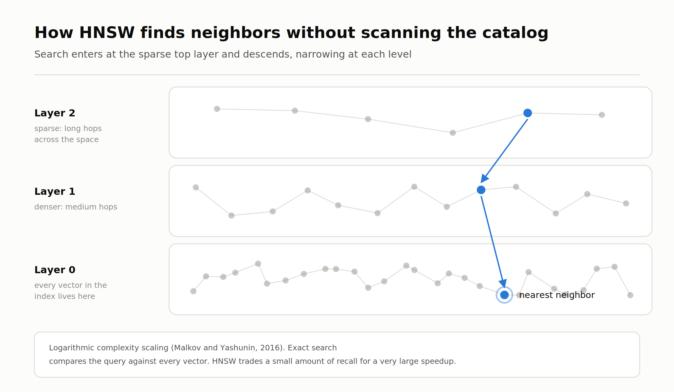
HNSW enters at the sparse top layer and descends, narrowing the candidate set at each level.

Storage is the constraint most teams underestimate. Taking pgvector’s documented layout as a reference, a vector column consumes 4 * dimensions + 8 bytes, with half-precision vectors at 2 * dimensions + 8 and bit vectors at dimensions / 8 + 8 (pgvector). Working that through for a one million SKU catalog at 768 dimensions:

Full precision: (4 × 768 + 8) × 1,000,000 = about 3.1 GB
Half precision: (2 × 768 + 8) × 1,000,000 = about 1.5 GB
Binary: (768 / 8 + 8) × 1,000,000 = about 0.1 GB

Those are raw vector bytes before index overhead, and they are arithmetic from a published specification rather than a measured benchmark. The point is the ratio, not the absolute figure. Note also that pgvector indexes the standard vector type up to 2,000 dimensions and halfvec up to 4,000, which quietly rules out some high-dimensional encoders if Postgres is the intended home.

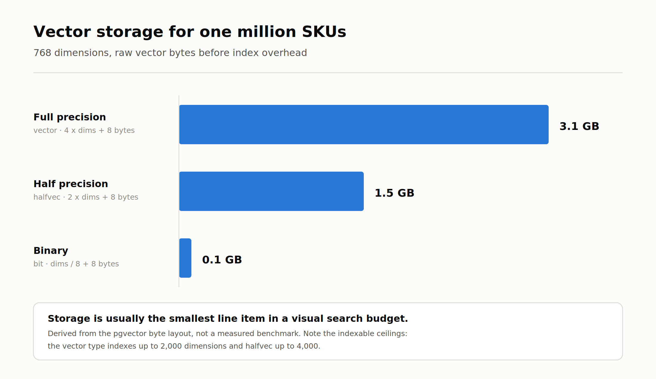
Raw vector bytes for a one million SKU catalog, derived from the pgvector byte layout. Index overhead is additional.

Binarization is not merely a storage trick. Pinterest reported that its unified embedding could be binarized for efficient storage and retrieval without compromising precision and recall, while a single multi-task embedding replaced several specialized ones and cut the operational cost of maintaining them (Zhai et al., Pinterest, KDD, 2019). eBay took a comparable route, using compact binary signatures to make latent space similarity tractable across a large and volatile inventory (Yang et al., eBay, KDD, 2017). Real-time image retrieval at catalog scale is as much a compression problem as a modeling one.

Why filtering belongs inside retrieval

This is where otherwise competent implementations fail, and it is almost never discussed.

Suppose the retrieval layer returns the top 50 nearest vectors, and the application then removes anything out of stock, outside the shopper’s shipping region, or outside the requested price band. If 48 of those 50 are filtered out, the shopper sees two results. If all 50 are filtered out, they see an empty page, and the system looks broken even though retrieval worked perfectly. This is post-filtering, and its failure rate rises exactly when the catalog is most constrained, which is to say during the sale periods when the feature matters most.

Pre-filtering inverts the order. Constraints are applied during the graph traversal or index scan so that only eligible items are ever considered as candidates. The top-k that comes back is a top-k of valid results. The cost is complexity: the index has to support attribute filtering natively, and highly selective filters can degrade graph traversal because the reachable neighborhood becomes sparse.

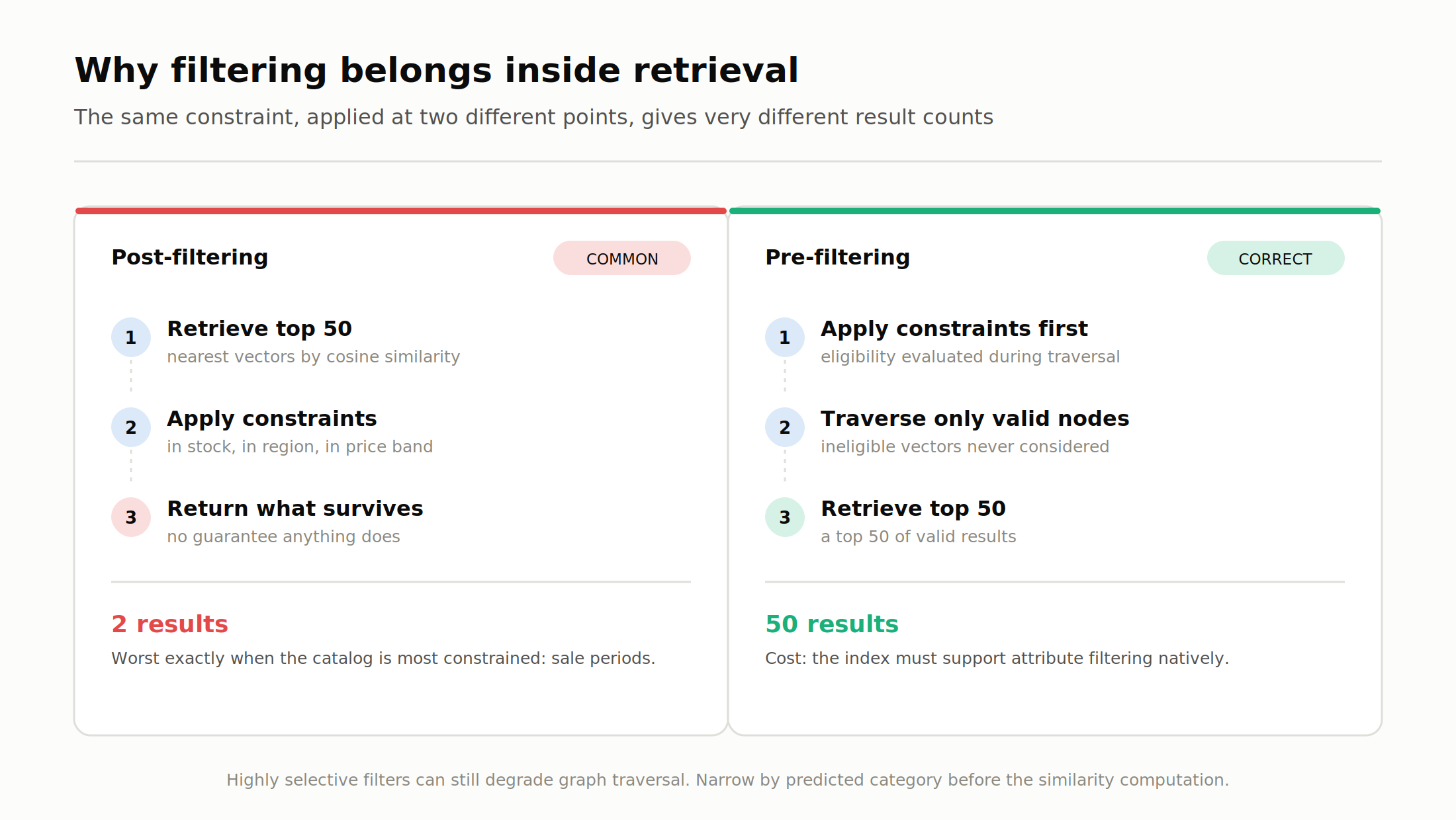
The same constraint applied at two different points in the pipeline produces very different result counts.

The production pattern that most reliably works is category filtering applied before the expensive similarity computation, which narrows the search space rather than discarding results after the fact. eBay’s system used a supervised approach that limited search to the top predicted categories, with a single deep neural network requiring only one forward inference, and the authors framed the design explicitly as a trade-off between search relevance and latency (Yang et al., eBay, KDD, 2017).

Category boundaries carry their own risk, though. Recent work on home goods visual search argues that coupling object detection to taxonomy-based classification makes systems dependent on catalog data that introduces noise, and proposes classification-free region proposals with unified embeddings instead. That approach was deployed on a global home goods platform and reported measurable uplift in customer engagement, with offline metrics correlating well with production outcomes (arXiv 2601.11769, 2026). The lesson for architects is that a taxonomy is a useful filter and a liability at the same time. If the catalog’s own categorization is inconsistent, filtering on it propagates that inconsistency into every search result. Cleaning that upstream is squarely an AI data engineering problem, not a model problem.

Re-ranking: where visual similarity stops being enough

The nearest vector is not always the best result. A visually perfect match that is discontinued, poorly reviewed, out of the shopper’s size, or carrying a thin margin is a bad outcome dressed up as a good one. Re-ranking is the stage where the system stops optimizing for visual similarity and starts optimizing for the outcome the business actually wants.

Re-ranking operates on a small candidate set, typically the top 100 to 500 from retrieval, which means it can afford computation that would be impossible across the full catalog. Three signal families usually feed it. Business rules encode hard commercial logic: suppress out-of-stock items, boost owned brands, respect merchandising overrides. Behavioral data brings click-through and purchase history for the specific product and for shoppers who submitted similar visual queries. Finer-grained visual scoring can apply a heavier cross-encoder that examines the query and candidate images jointly rather than comparing pre-computed vectors, catching detail differences that a single embedding smooths over.

Visual search personalization sits here too, and it deserves restraint. Personalizing too aggressively on a visual query undermines the shopper’s explicit intent. Somebody who photographed a specific object is expressing a very direct signal, and burying the closest match under items inferred from browsing history reads as the system ignoring them. The usual compromise is to keep the top few results driven by visual similarity alone and personalize the tail.

This stage is also where visual search connects to the wider recommendation surface. The candidates that lose the ranking are still relevant products, which makes them good inputs to Shop The Look style modules, shoppable pins, and shopping ads. Pinterest Lens and ASOS Style Match are two of the longest-running consumer implementations of that idea, and platforms including Instagram and TikTok have since built commerce surfaces on the same adjacency, where a visual query produces a purchase path rather than a single answer. Teams building the ranking layer on top of behavioral signals will find the modeling work overlaps heavily with predictive analytics.

What breaks in production

Three failure classes account for most of the distance between a convincing demo and a feature that survives contact with real traffic.

The domain gap. Catalog images are shot on white backgrounds with controlled lighting and a centered product. Shopper images are taken in living rooms, on sidewalks, at angles, under mixed lighting, with the item partly occluded. An encoder trained largely on clean web imagery produces embeddings for these two populations that sit further apart than the visual difference warrants. Object detection and cropping mitigate this by removing background before encoding. Fine-tuning on in-domain pairs helps more, but requires labeled pairs of user photos and their correct catalog matches, which most teams do not have on day one.

The variant problem. A product with twelve colorways generates twelve near-identical embeddings. Without deduplication, a single query can return one product twelve times and nothing else, which reads to the shopper as a broken search. The fix requires deciding whether to index at product level or variant level, and each choice has a cost. Product-level indexing with a canonical image loses the ability to match a specific color. Variant-level indexing preserves it but demands a dedup pass in re-ranking. On Shopify, variants can carry their own media and their own metafields, so the platform supports either strategy, and the architecture decision has to be made deliberately rather than inherited from whatever the catalog export happened to contain (Shopify).

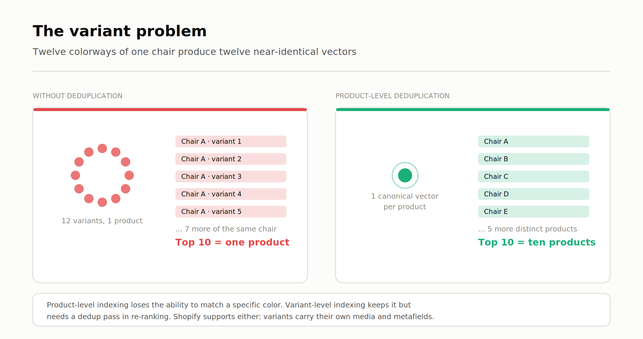
Without deduplication a single product can occupy every slot in the top ten.

Visual search cold start. A catalog below roughly a few hundred distinct products cannot reliably return a good match for an arbitrary query, because the nearest neighbor in a sparse space may still be visually unrelated. Presenting a confidently wrong result is worse than presenting none. Systems in this position need a similarity threshold below which they decline to answer and fall back to keyword search or category browsing.

A fourth risk is worth naming even though it is rarer in commerce. Adversarial visual perturbations, small changes to an image that are imperceptible to people but that move its embedding substantially, are a live concern for any visual system used in a trust or moderation context. Model versioning, reproducible reindexing, and monitoring of embedding drift are the operational answer, and they belong in the MLOps layer from the first release rather than being bolted on after the first incident.

Visual search in ecommerce catalogs

The model is the interesting part. The catalog is the hard part.

Every product image needs an embedding, and every embedding needs to reflect the catalog’s current state. A nightly CSV export was acceptable when visual search was a novelty. It is not acceptable when the feature drives search-driven revenue, because catalog sync latency turns directly into wrong results: products that sold out this morning still appear, products added this afternoon are invisible, and price or variant changes are stale.

The workable pattern is webhook-driven incremental re-embedding. When a product is created or its media changes, the system enqueues an embedding job and upserts the vector. When a product is unpublished or deleted, the vector is removed or flagged. Inventory status is best kept as a filterable attribute on the vector record rather than a reason to delete it, because stock returns and re-embedding is the expensive operation. Getting this right is ordinary data engineering discipline applied to a new data type, which is why native platform integration matters more than model selection for most merchants.

Category fit varies more than vendors usually admit. Fashion, home decor, furniture, jewelry, and accessories all have high visual variance that a shopper can perceive and cares about, which is what makes visual search useful. Commodities and consumables do not. Nobody photographs a bottle of dish soap to find a visually similar bottle of dish soap, because the distinguishing attributes are brand and volume, both of which are text. Scoping a visual search project to the categories where visual difference carries purchase intent is the single highest-leverage decision available before any code is written.

Product photography quality sets the ceiling on everything else. If catalog data contains images at inconsistent scale, with inconsistent backgrounds, or showing the product in a lifestyle context rather than isolated, embeddings inherit that inconsistency and unsupervised visual clustering of the catalog will group items by photographic style rather than by product. Auditing image consistency across SKUs before committing to a build usually reveals more about likely success than any model benchmark.

The scale that platform operators run at puts merchant catalogs in perspective. Google’s Shopping Graph holds more than 50 billion product listings, with more than 2 billion of those refreshed every hour (Google, 2025). No individual retailer needs that, but the refresh cadence is the instructive number: at that scale, freshness is treated as a continuous process, not a scheduled job.

Build or buy

The choice is between running an encoder yourself and calling a managed embedding API, and the honest answer depends on three variables that have nothing to do with model quality.

Volume and cost shape. Managed APIs price per image or per token and are inexpensive at low volume with no fixed cost. Self-hosting an open-weight encoder means provisioning inference capacity, which is a fixed cost that amortizes well at high and steady volume. The crossover point depends heavily on whether the workload is a one-time catalog backfill of millions of images or a steady trickle of query encodings. Many teams reasonably split the two, batching the backfill on rented GPU capacity and serving query-time encoding from a small always-on instance.

Latency and where inference happens. A visual search that takes three seconds to return will not be used twice. Query-time encoding sits directly in the user-facing path, so a network round trip to an external API is added latency that a local model does not incur. This is also the argument for edge-based visual search in mobile contexts, where running a compact encoder on the device removes the upload entirely and returns a vector instead of an image.

Data residency and privacy. Sending customer-submitted photographs to a third-party API is a data processing decision, not just a technical one. Visual search privacy deserves more attention than it typically receives, because user-submitted images frequently contain far more than the product: faces, interiors, documents, location cues. A system that retains query images for model improvement is making a commitment about that data, and that commitment needs to be documented, disclosed, and enforced. Self-hosting keeps images inside the perimeter, which for regulated industries can decide the question on its own. Where that decision needs formalising, our AI governance consulting practice handles the policy and audit side alongside the build.

A pragmatic sequence for most teams: start with a managed API to validate that visual search moves the metrics on a scoped category, then reassess self-hosting once volume is known and the cost shape is visible. Committing to infrastructure before demand is proven is the more expensive mistake. Deciding which path fits a given catalog and compliance posture is the kind of question our AI consulting engagements exist to answer.

How to measure whether it works

Visual search evaluation needs two separate measurement systems, and conflating them is why so many projects cannot say whether they succeeded.

Offline retrieval quality answers whether the system finds the right items. It requires a labeled relevance set: query images paired with the catalog items that a human judges correct. A few hundred queries with graded relevance is enough to start. Against that set, three metrics carry most of the signal. Recall@k measures whether the correct item appears in the top k at all, and it is the right metric for the retrieval stage because anything missed there can never be recovered by re-ranking. Mean average precision rewards putting correct results higher within the returned set. Normalized discounted cumulative gain handles graded relevance, distinguishing an exact match from a reasonable alternative from a miss, which suits visual search better than binary judgments because “similar” is genuinely a spectrum here.

Building that relevance set is unglamorous and is usually the step teams skip. Without it, every model change is a guess, and there is no way to know whether swapping encoders helped or hurt.

Online business impact answers whether finding the right items changed anything. Visual query volume, result click-through, add-to-cart rate, conversion rate from visual sessions, and revenue per visual session are the standard set. The comparison that matters is against the site’s existing search, on the same categories, over the same period.

A note on the numbers circulating about this. Specific conversion-lift figures for visual search are widely quoted, and the ones traceable to a source generally lead back to aggregator sites publishing no methodology, no sample size, and no date. Those do not survive a source check, so they are not repeated here. What can be said from primary sources is directional: platform operators have invested heavily in visual surfaces over a period when usage grew by roughly a factor of six in three years, which is a revealed preference rather than a marketing claim. Any team deciding whether to build should generate its own number from its own A/B test rather than inheriting one from a vendor blog.

Where Google is taking visual search

Watching how the largest visual search operator changes its architecture is a reasonable proxy for where the field is heading, and the direction is away from single-shot lookup.

Google’s visual search fan-out runs multiple background queries against one image to build a deeper understanding of its contents, combining Lens and Image Search with Gemini 2.5’s multimodal and language capabilities so the system recognizes subtle details and secondary objects rather than only the primary subject (Google, 2025). The framing from inside the team is that AI Mode performs roughly a dozen searches in the time a single search would take (Google, 2026).

That is architecturally significant. A fan-out over one image is a planning problem, not a retrieval problem. Something has to decide what the sub-queries should be, dispatch them, and synthesise the results into one answer. That control loop is the same pattern that shows up in AI agent development generally, and it suggests visual search is converging with agentic retrieval rather than remaining a specialized computer vision feature.

The second signal is multimodality becoming the default input rather than a mode. Google now describes searching across text, images, files, videos and browser tabs as inputs to the same system (Google, 2026). AI visual search from videos follows the same pipeline described in this guide, with frame sampling ahead of encoding, and query-by-sketch retrieval works because a sketch and a photograph can occupy one embedding space.

For teams building today, the practical read is to keep the layers separate. An architecture where detection, encoding, retrieval, filtering and ranking are distinct services can absorb a fan-out planner in front of it later. An architecture that fused them into one call cannot.

Frequently asked questions

What is the difference between AI visual search and reverse image search? Reverse image search finds copies or near-copies of a specific image, matching on visual fingerprints. AI visual search finds items that look similar without being the same image, using visual embeddings that capture semantic properties like shape, style and material. Reverse image search answers “where else does this exact picture appear.” Visual search answers “what else looks like this.” For a tool-by-tool comparison of what is actually available, see our guide to image search techniques.

How much data do you need before visual search works? There is no universal threshold, but the failure mode is well understood. Below a few hundred visually distinct products, the nearest neighbor to an arbitrary query may still be unrelated, and the system returns confidently wrong results. Small catalogs need a similarity threshold that declines to answer rather than returning the least-bad option.

Do you need to train your own model for visual search? Usually not to start. Pre-trained image embeddings from CLIP-family or SigLIP-family encoders transfer to unseen categories without task-specific training, which is what zero-shot capability means in practice. Fine-tuning becomes worthwhile once there are labeled pairs of real user queries and their correct matches, which only exist after the feature has shipped and collected traffic.

How long does it take to implement visual search on an ecommerce site? The variable is catalog readiness, not model integration. Calling an embedding API and standing up a vector index is days of work. Auditing image consistency across SKUs, deciding on product-level versus variant-level indexing, building webhook-driven sync, and constructing a relevance set for evaluation is where the schedule actually goes.

What does visual search cost to run? Costs fall into three buckets: one-time catalog backfill embedding, ongoing incremental embedding as the catalog changes, and query-time encoding plus vector search. Storage is usually the smallest line item. Using the pgvector byte layout, a million 768-dimension vectors is roughly 3.1 GB at full precision and roughly 1.5 GB at half precision, before index overhead.

Which product categories benefit most from visual search? Categories where visual difference drives purchase intent: fashion, home decor, furniture, jewelry and accessories. Categories where the deciding attributes are textual, such as commodities and consumables, gain little. Scoping to the right categories matters more than model choice.

Does visual search work better on mobile than desktop? Mobile is the native context because the camera is the input device, and the interaction of photographing an object and searching for it only exists there. Desktop visual search is generally upload or drag-and-drop from an existing image, which is a narrower use case. Mobile also enables on-device encoding, which removes the image upload from the request path.

Conclusion

AI visual search works by converting images into vectors and finding near neighbors, but that sentence describes maybe a fifth of the engineering. The rest lives in the pipeline around it: detecting the right object in a messy photo, choosing an encoder whose dimensionality the storage layer can carry, indexing approximately enough to be fast and exactly enough to be right, filtering before retrieval rather than after, and re-ranking on signals that visual similarity cannot see.

For ecommerce specifically, the binding constraint is almost never the model. It is whether the catalog can keep a vector index synchronized with a product set that changes hourly, and whether the categories in scope are ones where looking similar means being substitutable.

If visual search is on the roadmap, the highest-value work happens before any model is selected: audit image consistency across the catalog, pick the categories where visual difference carries intent, and build the labeled relevance set that will tell you whether any of it worked.

How Does AI Visual Search Work? A 2026 Engineering Guide